Markov-chain Monte Carlo on compact binary inspirals with spinning components

Parameter estimation

The goal of parameter estimation for gravitational-wave signals is to provide a statistically correct result for both the value of the source parameters and the accuracy of this determination. In order to do this, we determine the posterior probability-density function (PDF) of the unknown parameter set, given the data sets collected by a network of detectors and the prior information on the parameters. The probability is then provided by Bayes' theorem.

Markov-chain Monte Carlo

In order to compute the marginalised PDFs, we need to integrate over a large number of dimensions. Markov-chain Monte-Carlo (MCMC) methods are particularly effective in tackling these numerical problems. We developed an adaptive MCMC algorithm to explore the parameter space efficiently while requiring the least amount of tuning for the specific signal at hand. The challenge in this project is the large dimensionality of the parameter space for compact binary inspirals with spinning objects. Even for the case of a quasi-circular orbit, the number of dimensions in the parameter space considered is 12 for the case where one object is spinning and 15 for two spinning objects. We find that for the case of strong spin, the correlations between the parameters are strong, which makes the sampling of the parameter space less efficient and hence requires longer runs.

Sampling efficiency

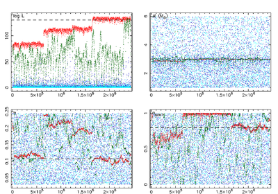
To sample a highly structured parameter space, it is necessary that the Markov chains cover both the entire space globally, and sample the local regions with high accuracy to get statistically useful results. The method we use in order to achieve this is parallel tempering in which 'hot' chains are more eager to accept jumps to lower likelihood and hence sample a broad range of the parameter space, whereas the 'cooler' chains are more reluctant to do so and make smaller jumps in more localised areas. When a hot chain stumbles upon a region with high likelihood, it can pass it down to the next cooler chain, until the regions with highest likelihood will be sampled in detail by the chain at the lower end of the 'temperature ladder'.

In the figure to the right (click for a larger version), the coolest chain is red, the hottest chain is cyan. The coolest chain finds the highest likelihood value (log(L), upper-left panel) after about 1.7×10⁶ iterations when the true values for both the symmetric mass ratio η (lower-left panel) and the dimensionless spin magnitude a_spin1 (lower-right panel) are found. The true value for the chirp mass M was already found after 6×10⁵ iterations (upper-right panel), when there was an earlier jump in log(L). The figure shows clearly how the cool chains sample a narrow region of interest (at high log(L)), while the hot chains explore the whole prior range of each parameter.

Convergence

A problem with MCMC in general is to determine when a Markov chain has converged. It turns out to be very useful to have several independent, serial chains running on the same data set, but starting from different locations in parameter space. When multiple chains agree on their results, both the parameter values and the corresponding value for the likelihood, then this is a strong indication of convergence in a (semi-)blind analysis. We compute the "R-hat statistic", in which the variances within chains are compared to the variances between chains in order to quantify convergence (Brooks & Gelman, 1998).

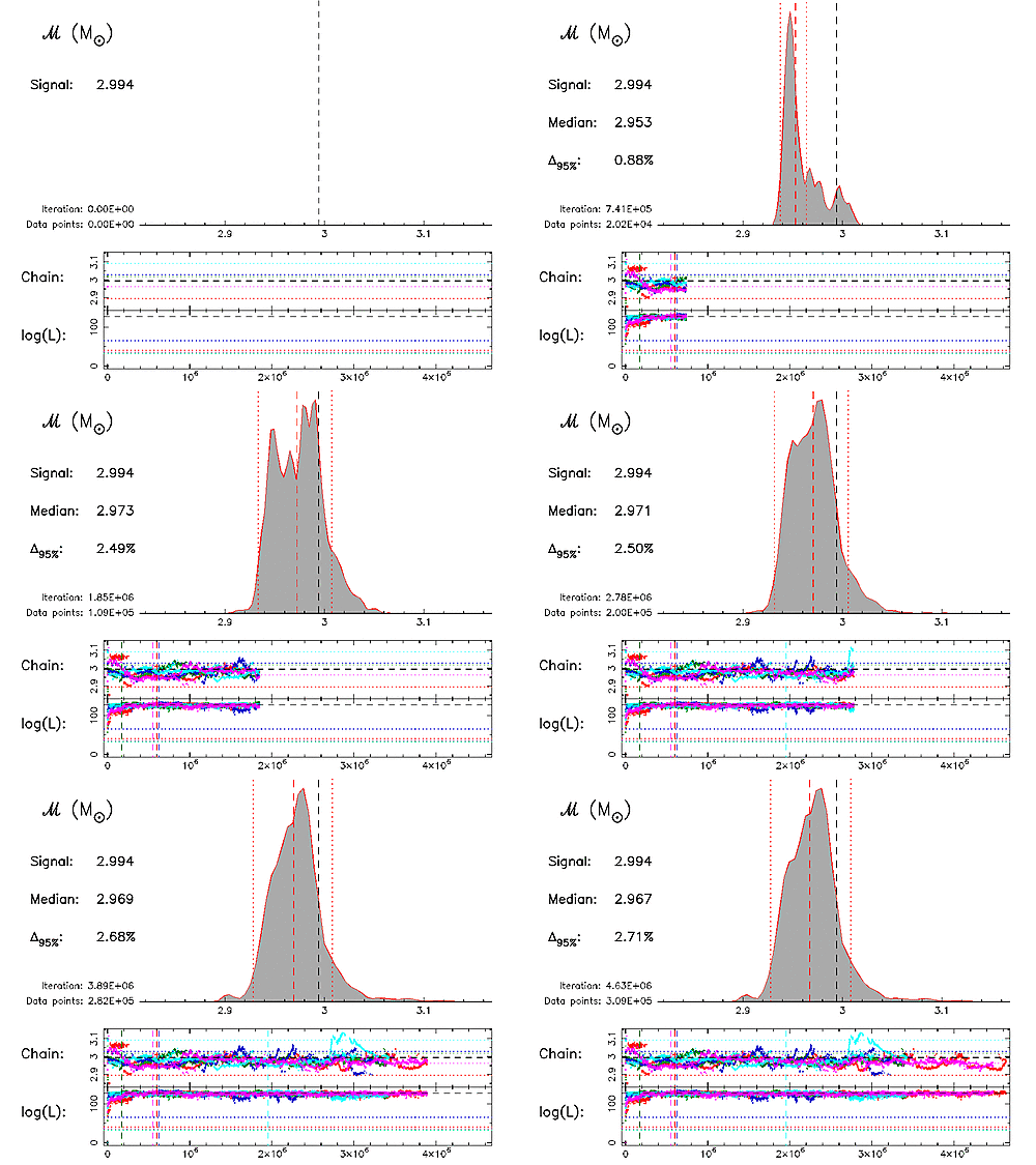
Example MCMC analysis

The animation to the left shows the output of a typical MCMC run with SPINSPIRAL, generated by AnalyseMCMC, using five serial chains (these are not communicating parallel chains with different temperatures, but the cool chains from five independent serial chains). The logarithm of the Likelihood (bottom panel) and the Markov-chain projection for the chirp mass (middle panel) are shown in a different colour for each chain. As soon as a chain has converged, a dashed vertical line is drawn in its colour to mark the end of the so-called burn in. All data points after the burn in are then included in the generation of the posterior probability-density function (posterior PDF, upper panel). The values to the left of the PDF show the chirp-mass values of the injected signal (black dashed line), the median of the PDF (red dashed line) and the 95% (or 2-σ) probability interval (Δ_95%, the region between the two red dotted lines). The animation shows that for a short run, with few data points, the PDF is very spiky. As more and more data points come in, the PDF becomes smoother, and the results converge. A larger version of this animation is available in MPEG format (71Mb).

A summary of the methods used in our MCMC code SPINSPIRAL was published in van der Sluys et al. 2008a; a paper with more technical details is in progress. A first example of astrophysically relevant results can be found in van der Sluys et al. 2008b.