AnalyseMCMC: reduction, analysis and presentation of SPINSPIRAL output

SPINSPIRAL is a Markov-chain Monte-Carlo code for the follow-up analysis of gravitational-wave signals from compact binary inspirals (black holes and neutron stars), as will be detected by LIGO and Virgo. AnalyseMCMC is a tool we developed for the reduction, analysis and presentation of the results from SPINSPIRAL. AnalyseMCMC generates one-dimensional and two-dimensional marginalised posterior probability-density functions (PDFs) for the 9, 12 or 15 parameters that describe the inspiral model (depending on whether 0, 1 or 2 spins are allowed for in the parameter estimation) and computes basic statistical properties.

The most important result from AnalyseMCMC is the indication of the best value, or a range of most likely values, for each parameter, or for combinations of parameters in the case of strongly correlated pairs (such as the two sky coordinates, or the individual masses). For single parameters, we can use the median and standard deviation to do this. However, we typically quote the 68%, 95% and 99% (“1-σ”, “2-σ” and “3-σ” respectively) probability ranges, i.e., the narrowest ranges that contain that percentace of the PDF, to indicate the uncertainty in our parameter estimation. For two-dimensional PDFs, this is more difficult. We estimate probability areas, but these are somewhat dependend on our choice of binning.

Example AnalyseMCMC output

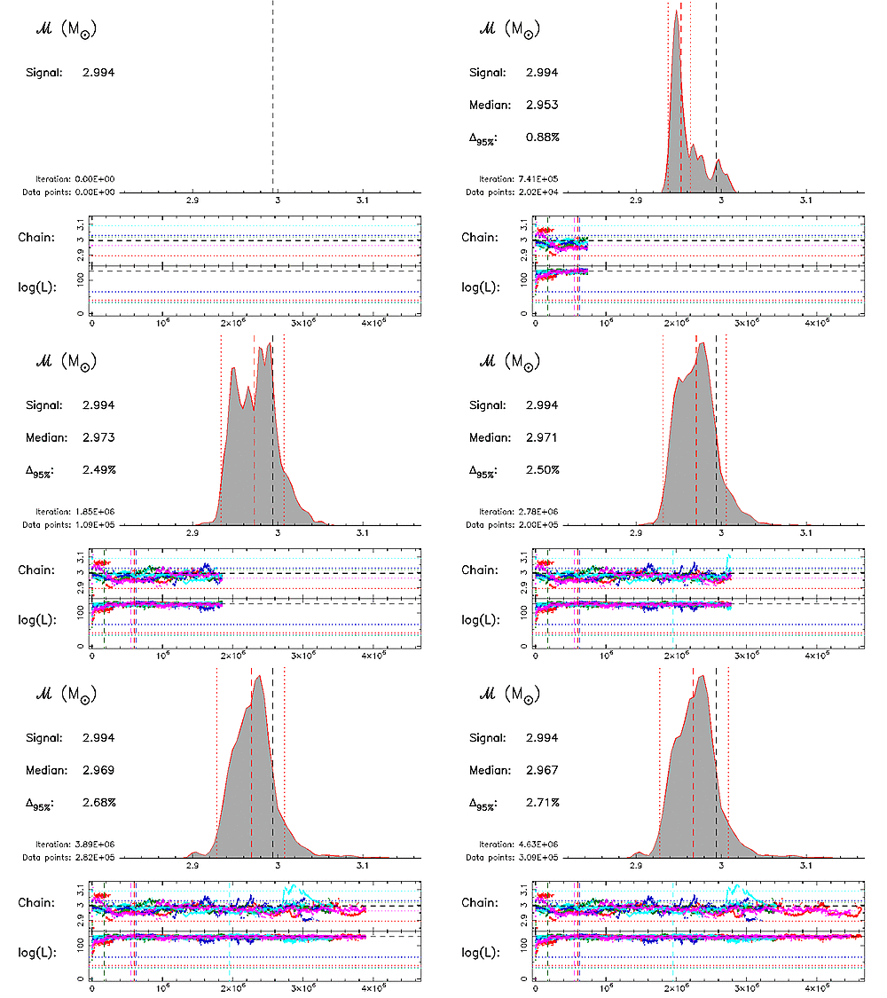
The animation to the right shows the output of a typical MCMC run with SPINSPIRAL, using five serial chains (these are not communicating parallel chains with different temperatures, but the cool chains from five independent serial chains). The logarithm of the Likelihood (bottom panel) and the Markov-chain projection for the chirp mass (middle panel) are shown in a different colour for each chain. As soon as a chain has converged, a dashed vertical line is drawn in its colour to mark the end of the so-called burn in. All data points after the burn in are then included in the generation of the posterior probability-density function (posterior PDF, upper panel). The values to the left of the PDF show the chirp-mass values of the injected signal (black dashed line), the median of the PDF (red dashed line) and the 95% (or 2-σ) probability interval (Δ_95%, the region between the two red dotted lines). The animation shows that for a short run, with few data points, the PDF is very spiky. As more and more data points come in, the PDF becomes smoother, and the results converge. A larger version of this animation is available in MPEG format (71Mb).

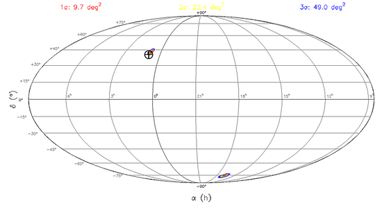
The figure to the left shows the two-dimensional marginalised PDF for the sky coordinates (right ascension α and declination δ), plotted on an all-sky map by AnalyseMCMC. The analysis was done using data from three non-colocated GW interferometers, and the resulting PDF is bimodal; the secondary (“false”) peak is located on the position of the primary peak, but mirrored in the plane spanned by the three detectors.

The three different colours of the PDF indicate the three probability ranges, and the numbers in the top of the figure show the corresponding areas in square degrees. The black symbol on the northern mode indicates the true location of the injected signal.

AnalyseMCMC source code and documentation